Combining research atlases with Earth observation data using natural language
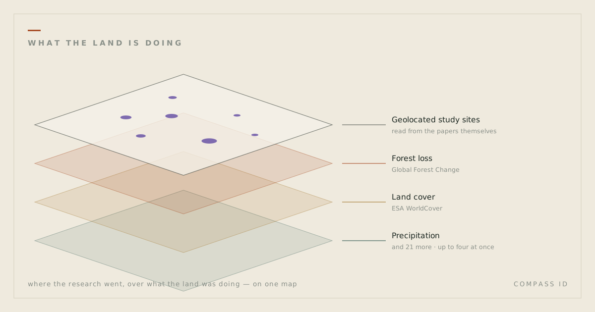
The interactive atlases now carry 24 Earth observation datasets from Google Earth Engine, drawn beneath the geolocated study sites. A request written in ordinary language is translated into a set of paper filters and a layer selection, which is what joins the two datasets. The model selects the view; it does not interpret the imagery.
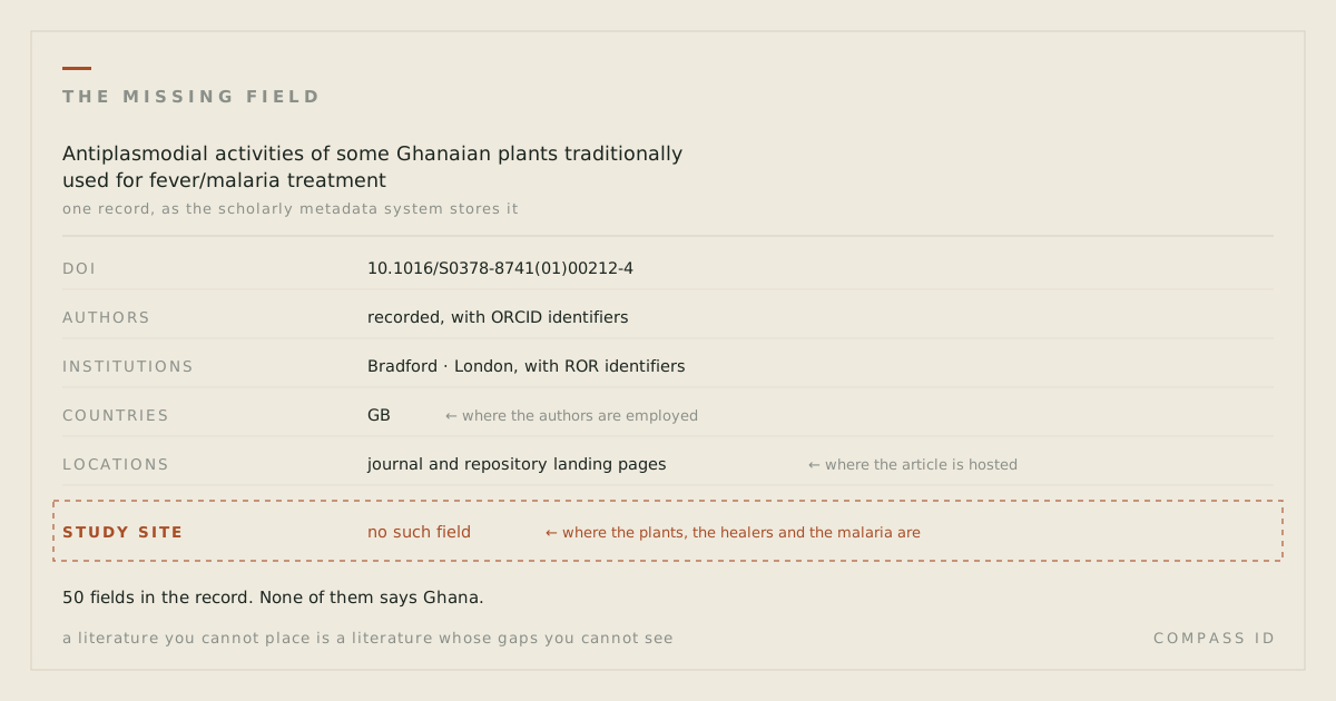
A COMPASS atlas reports where research has and has not been carried out. Each point is a study site extracted from the paper’s text, not the address of its authors. That answers one question and leaves a second one open: what environmental conditions hold at the sites where research is absent. Until now the atlas carried no data on that.
So the atlases now carry the second half: satellite-derived layers, 24 of them, served live from Google Earth Engine and drawn underneath the studies.
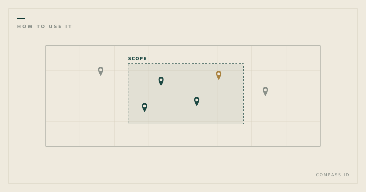
Combining them does not require knowing either dataset. A request such as show forest loss under the studies in Indonesia is resolved by the assistant into two things: a filter over the tagged literature, and a choice of raster layer. The datasets have no shared identifier, no shared vocabulary and no shared structure; location is the only attribute they hold in common, so location is what the join is made on. Translating the sentence into that pair of selections is the entire contribution of the language model here.
The datasets
- Land and vegetation: land cover, vegetation index, cropland extent, forest loss, biomass, mangroves, coral reef habitat, snow cover.
- Disturbance: active fires from the last 30 days, burned area, surface water change, land surface temperature.
- People: population density, night lights, human modification, protected areas.
- Air and climate: precipitation, soil moisture, sea surface temperature, aerosol index, nitrogen dioxide, carbon monoxide.
- Condition: the Biodiversity Intactness Index, and elevation as terrain context.
Up to four can be stacked at once, each with its own opacity and its own place in the stack, so you can fade one over another instead of flipping between them. Layers can be clipped to a single country, so a regional question does not get lost in a global picture. The whole arrangement is encoded in the URL, so a shared link opens the same map with the same layers in the same order.
Why combine them
When we published the desertification atlas, the central finding was that research effort and degradation burden are close to independent: rank dryland countries by how much research they host, rank them again by how badly degraded they are, and the two orders barely relate to each other (Spearman’s ρ ≈ 0). China alone holds more geolocated study sites (5,229) than the next six countries combined.
That correlation is a summary statistic. Displaying the degradation layer beneath the study sites shows the same relationship directly, at whatever spatial scale is of interest. The same comparison can be made with other layers: forest loss against the study sites of a plant family, to test whether research was carried out where forest cover was lost; or protected-area boundaries, to estimate what share of an evidence base was collected inside reserves. This is the sampling bias Martin, Blossey and Ellis reported in 2012, measured here on a specific corpus rather than assumed.
What the assistant will and will not do
It is worth stating precisely where that contribution ends.
The assistant does not report what the imagery shows. This constraint applies throughout the product: the model selects the view; the page computes every figure. The model receives no pixel values, so any statement it made about conditions at a site would be unsupported by evidence regardless of how plausible it read. Selection, filtering and layer choice are delegated to the model; interpretation of the imagery is not.
Legends and units
A colour ramp without a key cannot be read. Each of the 24 datasets therefore carries a legend in the sidebar, adjacent to the map: the palette as rendered, the measurement units, and the values at each end of the scale.
Where a layer is open to a specific misreading, the legend states it. Burned area is the clearest case: the ramp encodes the day of year on which a pixel burned, from 1 to 366. Darker values therefore indicate a later date, not greater severity. Four others carry similar notes. Nighttime radiance measures lit activity rather than population, so gas flares and lit fishing fleets register as bright while unlit settlements do not. The Biodiversity Intactness Index is modelled from land-use pressure, not observed from species counts. Active fires covers a 30-day window, so an empty area excludes anything that burned earlier. Tropospheric NO₂ is a whole-column retrieval at approximately 7 km resolution and is not equivalent to ground-level concentration.
Limitations
Spatial co-occurrence is not evidence of a relationship. Study sites overlying an area of forest loss establishes only that the two coincide in space. It does not establish that the studies concerned forest loss, or that either is causally related to the other. The overlay is a basis for further examination, not a result.
The spatial resolutions are not comparable. A study site is a point; the atmospheric products are on grids of roughly 7 km and the reanalysis soil-moisture product roughly 11 km. Point-to-cell comparison at that disparity is adequate for orientation and inadequate for inference. Coarse resolution is stated in the legend of each affected layer.
The Earth observation layers are available on all five interactive atlases. They are drawn beneath the study sites; the research coverage remains the subject of the map and the environmental data is context for it.